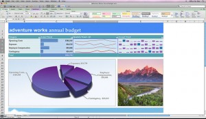
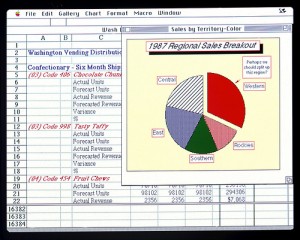
These days a critical job skill for Success in almost any position other than manual labor or minimum wage jobs is computer skills. Basic computer skills involves wordprocessing (like Microsoft Word®) or other Office Programs like MS Excel®, Powerpoint, etc. In this article we are going to look at a skill that every job seeker should have and that is using Microsoft Excel®. After learning how to enter data into rows and columns one of the next things you will want to do is create a chart using Microsoft Excel®.
Steps By Step Guide To Create a Chart/Graph in MS Excel®
Microsoft Excel® has been widely used around the world as a business application for storing, organizing and manipulating the data of the organization in a systematic format. Nowadays, the use of excel is not only restricted to business uses, but is also used by students and professionals for everything from playing music to training pilots. Despite of availability of other specific use software, people still consider using rows and columns to manage data. This is because the various features and applications offered by excel are familiar, easy to use and readily available.
One easy to use function is the creation of pie charts, graphs and other comparative presentations in Excel. To learn all the key aspects of using excel, you do not need any special training. In this article, we will tell you the step by step procedure to create graphical representations in MS Excel® 2010.
Steps to Create Charts/Graphs in MS Excel®
Step 1 – The first step is to launch Excel on your desktop. Simply click on the Start Menu > All Programs > Microsoft Office> Microsoft Excel. Now to begin your work, open a new spreadsheet. It can be done in three ways:
1. Go to the File menu. Select New.
2. Go to the Standard toolbar. Click on the New Workbook button.
3. Use a keyboard shortcut: Ctrl + N on a Windows computer.
Step 2 – Enter the data on the spreadsheet you want to graph. You can also import the data from other spreadsheets as well.
Step 3 – Highlight or select the data that is to be graphed. Do not include the row with heading and titles. Put your cursor on the second row, first column (A2:C1), hold the mouse button and drag to the point where you want to create the graph.
Step 4 – Click on the Insert Menu and select “Chart Wizard” option. You can also click on the Chart Wizard button given on the Standard toolbar.
Step 5 – A new window will open as soon as you will click on the Chart Wizard. Now select Chart type from the given option. For instance: you can select pie chart option. Once you have made the selection, click and hold your mouse pointer down on the Press and Hold to see the preview of your data.
Step 6 – Select “Next” and a new window will get opened showing you a series of options you a series of options consisting of colours, size, etc. to make changes to your chart.
Step 7 – Click on “Finish” and the Chart Wizard will puts your completed chart on the spreadsheet.
Step 8 – You can add labels, legends, title on the chart by clicking on the dialogue box given at the end of the chart. Moreover, the dialog box will shrink allowing you to edit the data range in this small window.
Creating a chart on a spreadsheet is not at all difficult. It does not matter if you are familiar with the older versions of Microsoft Office, you can easily perform all these steps on MS Excel 2010, without undergoing any excel 2010 training. Other Excel versions will create a Chart in a similar manner i.e they don’t have major differences in respect to the commands, and methods. But they may have slightly different features for the finished chart.
Take a few minutes to practice creating charts in Excel and modifying them to get the look you desire. It will be a useful skill to develop.
See Also:
Choosing a Professional Resume Writing Service
Group Health Insurance Policies
What to Look for in an Online Degree Program
The Difference a Degree Makes in Unemployment Levels
10 Awesome Jobs You Can Do From Home
About the Author:
This article was contributed by http://www.exceleverest.com/
Photo Credits: Microsoft Sweden


